Feature Validation
This section has to do with the predictions done on the initial dataset in an attempt to view how accurate the model is and to prove findings.
First we train the perceptron and SVC with continuous data and convert the different student levels to vectors as shown below.
df['TotalQ'] = df['Class']
df['TotalQ'].loc[df.TotalQ == 'Low-Level'] = 0.0
df['TotalQ'].loc[df.TotalQ == 'Middle-Level'] = 1.0
df['TotalQ'].loc[df.TotalQ == 'High-Level'] = 2.0


X = np.array(continuous_subset).astype('float64')
y = np.array(df['TotalQ'])
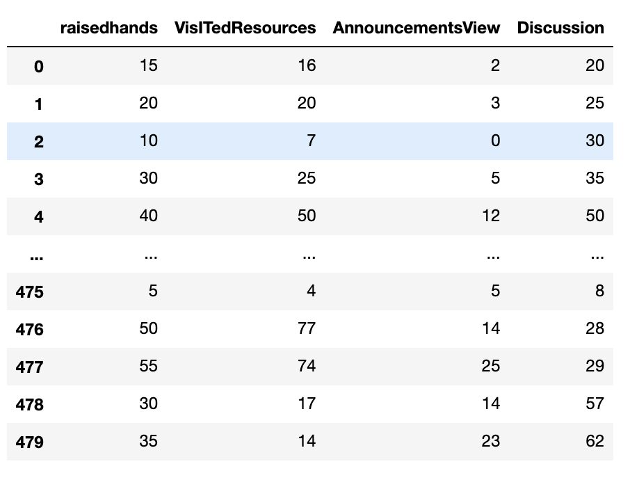
Here we gain a look at the continuous subset with 4 of the features we had chosen using a dataset of 479 students.

We then use sklearn preprocessing to and model selection to get a train split and a test split as well as scale the data
from sklearn.model_selection import train_test_split
from sklearn.preprocessing import StandardScaler


X_train, X_test, y_train, y_test = train_test_split(
         X, y, test_size=0.3, random_state=0)


sc = StandardScaler()

sc.fit(X_train)

X_train_std = sc.transform(X_train)
X_test_std = sc.transform(X_test)
From here on we initially got an accurace of 47% on training with just the perceptron. The misclassified samples were 76 out of the test split.
The perceptron initially gave the lowest training percentage.
Next we used the linear SVC to train the model
from sklearn.svm import SVC

svm = SVC(kernel='linear', C=2.0, random_state=0)
svm.fit(X_train_std, y_train)

y_pred = svm.predict(X_test_std)
This garnered an accuracy of 64% with 52 misclassified samples.
We then added the field for the absence days to the continuous dataset and trained it again using the linear SVC and after getting an accuracy of 77% we store the model using pickle and then use the file to serve our learning adaptation platform.
svm.fit(X_train_std, y_train)

y_pred = svm.predict(X_test_std)
filename = 'svm.sav'
pickle.dump(svm, open(filename, 'wb'))